Today we’ll talk about FAIRS’s paper: Understanding Training Efficiency of Deep Learning Recommendation Models at Scale.

---

Overview

In this paper, Facebook researchers experiment on and analyze the training stage of large recommender systems. This goes from hardware consideration to embedding strategies. From data representation considerations to task distribution policy. Their goal is to be able to provide a more in-depth understanding of what can affect the speed and accuracy of a large production recommendation model. Namely, they compare the use of three different hardware set-ups in use at Facebook, to train three of their large-scale recommender systems. They chose those specific three models to compare as their specificities are quite different from one to another and allow one to better understand what is to be taken into consideration before defining a deployment policy.

Facebook ML training

Before we jump into the experiments, let us first have a look at some facts on ML training. Facebook uses a custom infrastructure for their model training and use several types of machines for that purpose.

Generic background

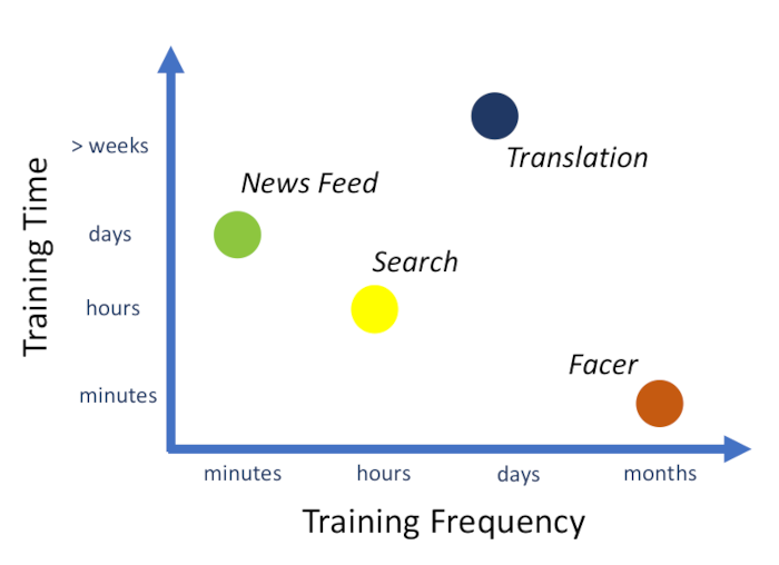
Facebook routinely trains a high number of models for its different services. They all have different training times and frequencies depending on the specific requirements. It is therefore important that training times are kept low to reduce resource utilization in the long run, as well as avoiding the deployments of already stale models may they take too long to train.

In our case, the authors describe three major steps in the training of a recommendation model at Facebook.

1. Data fetching and pre-processing
2. Actual training (we will focus on this one)
3. Model deployment

To tackle the challenge of performing that many training runs, Facebook developed its GPU-based architecture called Big Basin. This architecture was not tailored to recommendation model handling. Therefore, their hardware requires extra care for an efficient strategy for the serving of embedding tables in the context of recommender systems.

Recommendation model specificities

To understand what may affect the training performances of those models, the authors first summarize their two main components. Embedding layers used to represent categorical features by dense vectors and multi-layer perceptrons used to represent continuous features. Both components are used to learn latent space representation of their respective features which are then used by the rest of the model. For the MLP components, each trainer holds a copy of the model during training and regularly updates it with the rest of the workers. The problem with the embeddings table can’t be solved this way. As there is a potentially very high number of embeddings to store in memory, it is not possible to fit them all into a single machine. There is therefore a partition of those embeddings across different embedding servers. Those servers store only a fraction of all embeddings and thus are called sparse parameter servers.

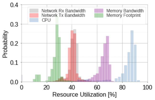
When looking at training performance, one might look at resource usage. In our case CPU, memory, and network usage. It happens that these usages resemble a gaussian distribution with its parameters depending on the model’s characteristics and configuration. In the figure below, we see the distribution of resource utilization of multiple train runs of the same model in the same environment but with different parameters. The authors suggest that the variability in the distributions comes from these differences in parameters as well as some system-level variability. That means that while not being totally predictable, model training runs behave consistently in their resource utilization. Therefore, it makes sense to look for the most suitable hardware when deploying those ML models to production.

Hardware considerations

In the following experiments, three distinct hardware setups will be used.

1. The first one is a two CPU machine and is called the dual-socket.
2. The second is composed of 2 CPUs and 8 V100 GPUs interconnected using NVLINK and is called Big Basin and offers about 900 GB/s of bandwidth.
3. The third machine is made of 8 CPUs and 8 GPUs and offers a whopping 2 TB/s of bandwidth and is called Zion.

Each of those setups requires a custom configuration of the software running it. Therefore each of them has to get their configuration tuned before being able to properly compare them. Examples of these parameters to set are the number of working and data loading threads, embedding placement strategy, and the number of workers. We will describe here the different placement strategies explored in the paper.

The first and obvious strategy is to solely use the GPU memory to store embeddings. This will favor systems with lower GPU-CPU bandwidth. In the case where the table does not fit into the GPUs memory, the inter-worker communication becomes the primary bottleneck.

The second method is to use the CPU memory. In that case, a lot of CPU-GPU copies have to be made. Therefore, only systems with high GPU-CPU bandwidth will be able to perform well. Here, the CPUs can become a bottleneck as they will have to bear the load of all copies being made.

The third approach is to store the embeddings on remove CPU memory. This will tackle the bottleneck seen in the previous approach as it enables the scaling of the number of CPUs handling the operations on embeddings. However, it also increases latency as networking is involved.

Last but not least, a hybrid approach can also be used where some embeddings are stored on the GPU memory and some others are stored on the CPU side. In that case, the stress on CPUs is partially relieved as part of their workload is directly handled by the GPUs.

The efficiency of various model configurations

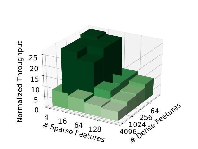
The different architectures seen above are tested using different combinations of the number of sparse and dense feature pairs. The intuition behind it is that the lower the number of features used by the model, the higher the throughput. Let us get a feeling of their findings through the following figures:

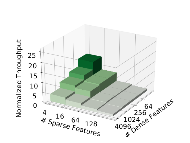
The figure above represents the throughput of the model training according to both the number of sparse and dense features on CPU. We can see that past 64 sparse features, the model sees a huge hit in performance. This is probably due to the fact that the embeddings no longer fit into single host memory and increased usage of networking is required.

In this figure, we see that the GPU-based throughput is higher no matter what. Again we see a clear step in throughput as the number of features varies.

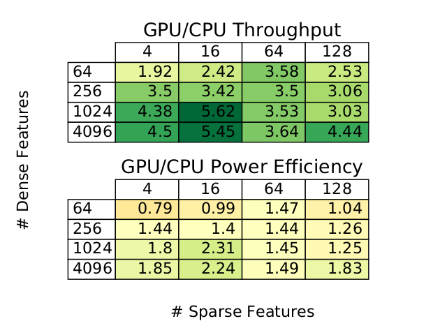
The authors note that on average, Big Basin consumes 7.3 times more power than the CPU system. This means that the power efficiency isn’t necessarily better for GPU workers. In the figure above, we see that for the lowest number of features, the CPU consumes less power to train. We even see that the less dense features occur in a worse performance of the GPU relative to the one of the CPU.

Another interesting finding of the paper is the different relations between the hash size and throughput. Hash tables are used to limit the set of possible sparse feature values. The higher the hash size is, the more possible embedding values become possible. Of course, a large number of embeddings means a lot of memory consumption. In our case, several hash sizes are tested on both CPU and GPU architectures.

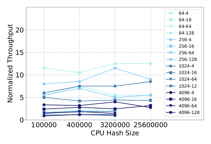
In this first figure, the different lines correspond to different combinations of the number of sparse and dense features. we can observe that the throughput remains “stable” no matter what the hash size is. No clear correlation can quickly be observed here. The explanation of the authors is simple. For all experiments shown here, the host memory was enough to store the embeddings.

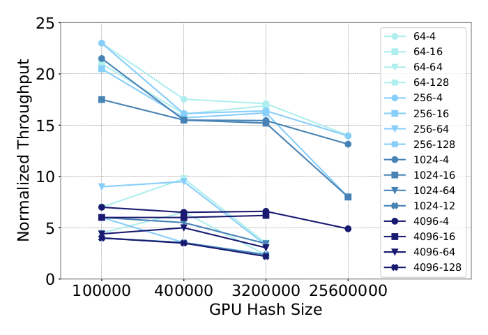
In this second figure, however, things are different. We can see that as the hash size grows, the throughput does take a hit. We can even see that the higher the throughput values are, the bigger the hit is. In this case, as the hash size is growing, the number of GPU required to store the embeddings grows alongside the inter-GPU communications. This is why we see such a dramatic drop in throughput here.

Real world efficiency

To conclude this overview, we will look at some insights collected on some real models used in production at Facebook. They all present different characteristics and we’ll see that choosing the hardware and the memory placement strategy isn’t straightforward at all.

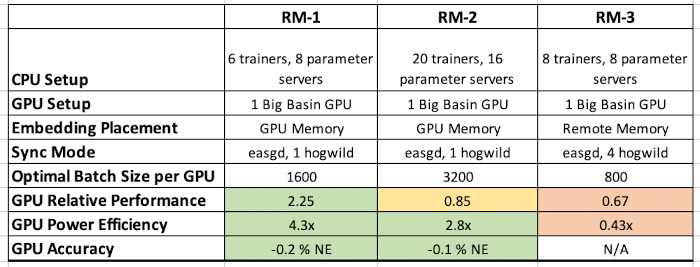
This first column presents results for the M1 model. It has a low number of sparse features but a high number of dense features. Its embedding table size is in the order of tens of GB. These characteristics are perfect for a GPU system as they perform really well on dense features and when the memory consumption is limited. We see that the GPU is better in both throughput and training efficiency.

The second column presents the model M2, which has similar characteristics to the M1 except for the number of dense features where it is low. This lower number of dense features is enough to reduce the edge GPUs have and make CPU systems actually faster than the GPU system at this task. It is interesting to note, however, that despite being slower, the GPU system still presents a better power efficiency.

The last column presents the model M3. M3 has a high number of both sparse and dense features, its embedding table size is in the order of hundreds of GB which makes it way heavier than the two previous models. As we have seen previously, this memory consumption causes a lot of problems for the GPU as there have to be a lot more data copies. This considerably impacts the performance of the model on GPU systems and makes it both faster and more power-efficient to train on CPU systems.